Connecting to FRED Data
Reading in Data From FRED
#install.packages("modelr")
#install.packages("FinCal")
#install.packages("dplyr")
#install.packages("FinancialMath")
#install.packages("devtools")
#install.packages("tidyverse")
#install.packages("dplyr")
#install.packages("ggpubr")
#install.packages("epitools")
#install.packages("data.table")
#install.packages("usmap")
#install.packages("maps")
#install.packages("cowplot")
#install.packages("ztable")

library("modelr")
library("FinCal")
library("dplyr")
##
## Attaching package: 'dplyr'## The following objects are masked from 'package:stats':
##
## filter, lag## The following objects are masked from 'package:base':
##
## intersect, setdiff, setequal, unionlibrary("FinancialMath")
library("ggplot2")
library("quantmod")## Loading required package: xts## Warning: package 'xts' was built under R version 3.5.2## Loading required package: zoo##
## Attaching package: 'zoo'## The following objects are masked from 'package:base':
##
## as.Date, as.Date.numeric##
## Attaching package: 'xts'## The following objects are masked from 'package:dplyr':
##
## first, last## Loading required package: TTR## Warning: package 'TTR' was built under R version 3.5.2## Version 0.4-0 included new data defaults. See ?getSymbols.##
## Attaching package: 'quantmod'## The following object is masked from 'package:FinCal':
##
## lineChartlibrary("epitools")## Warning: package 'epitools' was built under R version 3.5.2library("data.table")## Warning: package 'data.table' was built under R version 3.5.2##
## Attaching package: 'data.table'## The following objects are masked from 'package:xts':
##
## first, last## The following objects are masked from 'package:dplyr':
##
## between, first, lastlibrary("usmap")## Warning: package 'usmap' was built under R version 3.5.2library("maps")
library("cowplot")## Warning: package 'cowplot' was built under R version 3.5.2##
## ********************************************************## Note: As of version 1.0.0, cowplot does not change the## default ggplot2 theme anymore. To recover the previous## behavior, execute:
## theme_set(theme_cowplot())## ********************************************************library("ztable")## Welcome to package ztable ver 0.2.0Connecting to FRED through an R package downloaded from GitHub
US GDP from Jan 1st, 1990 to today
#See https://fred.stlouisfed.org/docs/api/fred/ for FRED Data information


#See https://fred.stlouisfed.org/tags/series for series IDs
fredr(series_id = "UNRATE",
  observation_start = as.Date("1990-01-01"))
## # A tibble: 367 x 3
## date series_id value
## <date> <chr> <dbl>
## 1 1990-01-01 UNRATE 5.4
## 2 1990-02-01 UNRATE 5.3
## 3 1990-03-01 UNRATE 5.2
## 4 1990-04-01 UNRATE 5.4
## 5 1990-05-01 UNRATE 5.4
## 6 1990-06-01 UNRATE 5.2
## 7 1990-07-01 UNRATE 5.5
## 8 1990-08-01 UNRATE 5.7
## 9 1990-09-01 UNRATE 5.9
## 10 1990-10-01 UNRATE 5.9
## # … with 357 more rows#US GDP from Jan 1st 1990 to now
GDP <- fredr(series_id = "GDP",
observation_start = as.Date("1990-01-01"))
GDP %>%
ggplot(aes(x = date, y = value)) +
geom_line() +
ggtitle("GDP for US in Billions of Dollars") +
labs(x = "Date", y = "Billions of Dollars")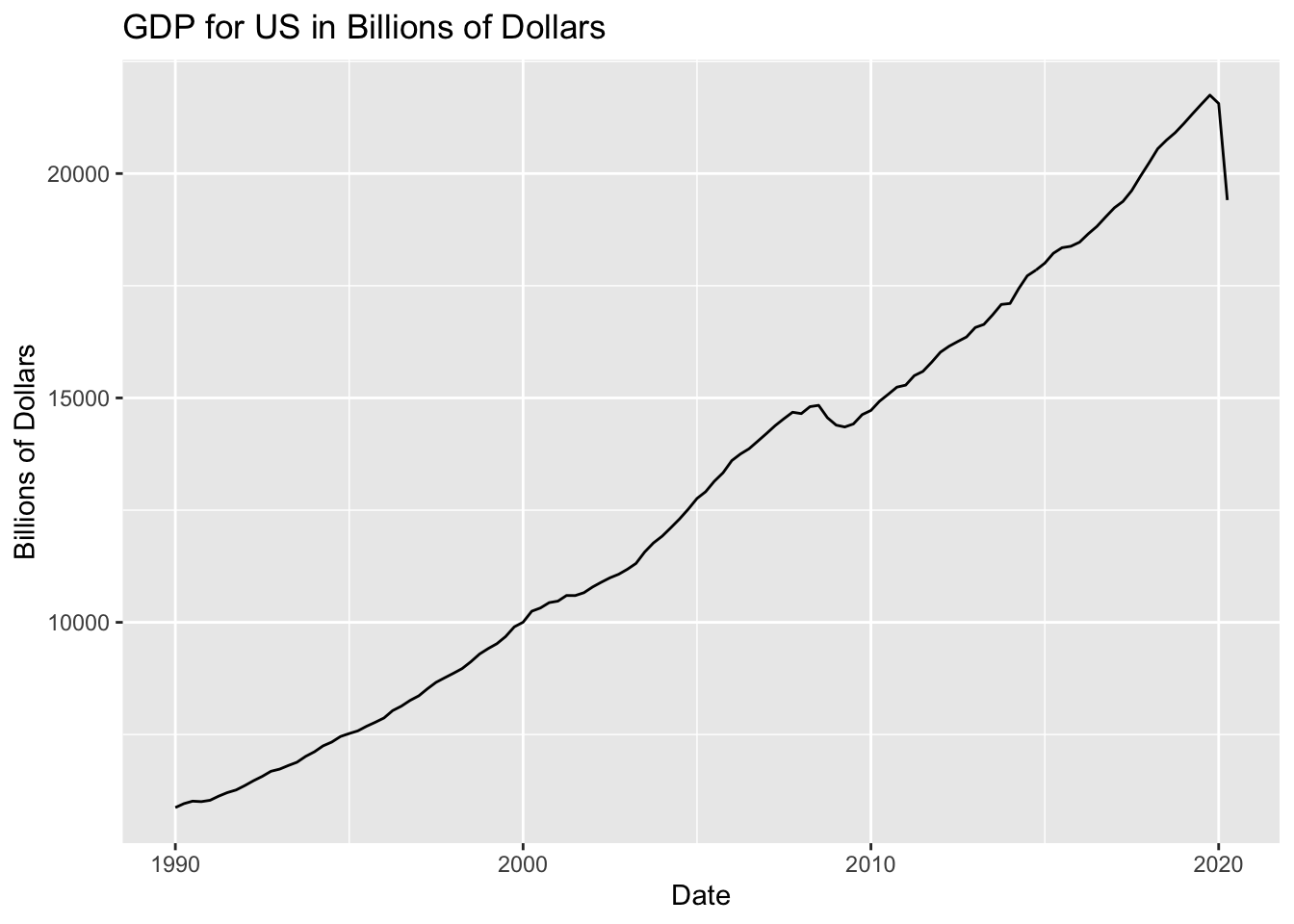 [Us GDP has steadily increased since 1990 with slight deviations from norm in 2009 and most recently 2020. 2009 deviation explained by 2008 financial crisis, and 2020 deviation explained by the COVID pandemic.]
Percentage Change in Richmond, Virginia Poverty Rate since January 7,1990
#Change in Richmond, Virginia Poverty Rate since January 7,1990
RVA_POV <- fredr(series_id = "S1701ACS051760",
  observation_start = as.Date("2013-01-01"),
  frequency = "a")

RVA_POV %>%
  ggplot(aes(x = date, y = value)) +
  geom_line()  +
  ggtitle("Poverty Rate for Richmond VA") +
  labs(x = "Date", y = "% of Population")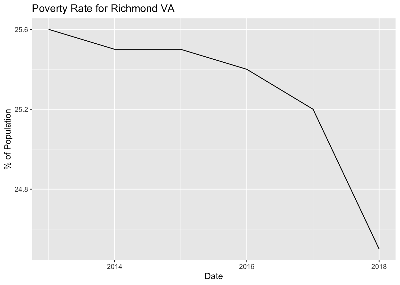
[Poverty Rate in Richmond, Virginia has decreased since 2013 from 25.6% to 24.5%. With an economy that improved substantially during this time period, this observation doesn’t seem difficult to imagine]
#Home ownership rate for Virginia
VA_Home <- fredr(series_id = "VAHOWN",
observation_start = as.Date("1984-01-01"),
frequency = "a")
VA_Home %>%
ggplot(aes(x = date, y = value)) +
geom_line() +
ggtitle("Home Ownership in VA") +
labs(x = "Date", y = "% in Population")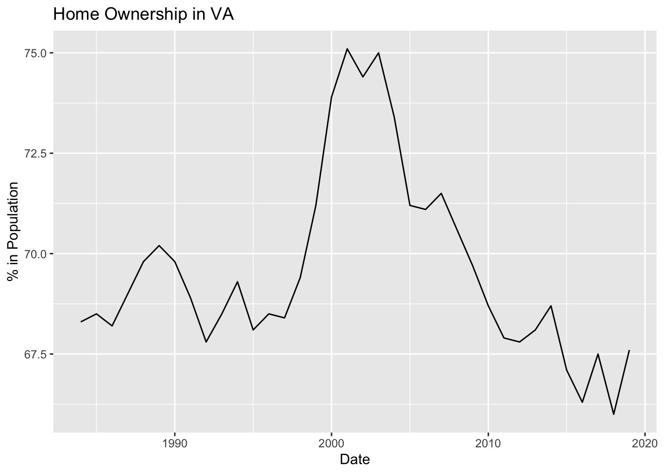 [Home Ownership in Virginia appears to have peaks in 1989, 1994, 2001, 2003, 2007, 2013, 2017 and 2019. From this visualization you can clearly see the the housing bubble in the early 2000s that led to the 2008 financial crisis. Home ownership appears to have a slight decline since 2007.]
Correlation Analysis of TIPS Interest Rates and NYSE Stock Prices
#Daily Interest Rates for 10 Year Treasury Inflation Indexed Securities
T_INT_RATES <- fredr(series_id = "DFII10",
  observation_start = as.Date("2003-01-02"),
  frequency = "d")

#Daily Stock Data is downloaded using quantmod
DJI <- getSymbols("DIA", src = "yahoo", from = '2003-01-02', to = "2020-07-31", auto.assign = TRUE)
## 'getSymbols' currently uses auto.assign=TRUE by default, but will
## use auto.assign=FALSE in 0.5-0. You will still be able to use
## 'loadSymbols' to automatically load data. getOption("getSymbols.env")
## and getOption("getSymbols.auto.assign") will still be checked for
## alternate defaults.
##
## This message is shown once per session and may be disabled by setting
## options("getSymbols.warning4.0"=FALSE). See ?getSymbols for details.DIA_Daily_Return <- dailyReturn(DIA)
#Daily Stock Prices are Plotted
DIA_Daily_Return %>%
ggplot(aes(x = index(DIA_Daily_Return), y = daily.returns)) +
geom_line(size=0.5, color="steel blue") +
ggtitle("Daily Return for Dow Jones ETF since 2003") +
scale_x_date(date_breaks = "years", date_labels = "%Y") +
labs(x = "Date", y = "Adjusted Price")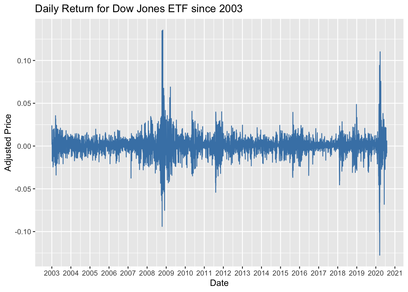
#Left Join by Date
DIA_Daily_Return <- data.frame(DIA_Daily_Return)

DIA_Daily_Return$date <- as.Date(rownames(DIA_Daily_Return))

T_INT_RATES$TIPS_Rate <- T_INT_RATES$value

Int_Rate_Stock_Data <- merge(x = DIA_Daily_Return, y = T_INT_RATES, by = "date", all.x = TRUE)

head(Int_Rate_Stock_Data)
## date daily.returns series_id value TIPS_Rate
## 1 2003-01-02 0.0241235645 DFII10 2.43 2.43
## 2 2003-01-03 0.0020886633 DFII10 2.43 2.43
## 3 2003-01-06 0.0151690248 DFII10 2.46 2.46
## 4 2003-01-07 0.0005703548 DFII10 2.42 2.42
## 5 2003-01-08 -0.0176698926 DFII10 2.29 2.29
## 6 2003-01-09 0.0186840088 DFII10 2.41 2.41cor.test(Int_Rate_Stock_Data$daily.returns, Int_Rate_Stock_Data$TIPS_Rate)##
## Pearson's product-moment correlation
##
## data: Int_Rate_Stock_Data$daily.returns and Int_Rate_Stock_Data$TIPS_Rate
## t = -0.59466, df = 4391, p-value = 0.5521
## alternative hypothesis: true correlation is not equal to 0
## 95 percent confidence interval:
## -0.03853599 0.02060440
## sample estimates:
## cor
## -0.008973643[Similarly, this analysis was done to try to determine if there was a strong correlation between the Dow Jones and Interest Rates for 10 Year Treasury Inflation Indexed Securities. The thought behind this was increased TIP rates signaled an improving economy thus causing an increase in the price of the Dow Jones Index and in this case an ETF. With a P value above the .05 threshold there is not enough evidence to suggest a relationship exists.]
Correlation Analysis of TIPS Interest Rates and GDP
#Daily Interest Rates for S&P/Case-Shiller U.S. National Home Price Index
HPI <- fredr(series_id = "CSUSHPINSA",
  observation_start = as.Date("2003-01-02"),
  frequency = "m")

#Daily Stock Data is downloaded using quantmod
DJI <- getSymbols("DIA", src = "yahoo", from = '2003-01-02', to = "2020-05-31", auto.assign = TRUE)

DIA_Monthly_Return <- monthlyReturn(DIA)

#Left Join by Date
DIA_Monthly_Return <- data.frame(DIA_Monthly_Return)

DIA_Monthly_Return$date <- seq(as.Date("2003/1/1"), as.Date("2020/5/31"), by = "month")

HPI$index <- HPI$value

HPI_Stock_Data <- merge(x = DIA_Monthly_Return, y = HPI, by = "date", all.x = TRUE)

head(HPI_Stock_Data)
## date monthly.returns series_id value index
## 1 2003-01-01 -0.039334592 CSUSHPINSA 127.652 127.652
## 2 2003-02-01 -0.018926250 CSUSHPINSA 128.327 128.327
## 3 2003-03-01 0.006430488 CSUSHPINSA 129.310 129.310
## 4 2003-04-01 0.063142082 CSUSHPINSA 130.490 130.490
## 5 2003-05-01 0.046900718 CSUSHPINSA 131.841 131.841
## 6 2003-06-01 0.012044215 CSUSHPINSA 133.226 133.226cor.test(HPI_Stock_Data$monthly.returns, HPI_Stock_Data$index)##
## Pearson's product-moment correlation
##
## data: HPI_Stock_Data$monthly.returns and HPI_Stock_Data$index
## t = -0.44315, df = 207, p-value = 0.6581
## alternative hypothesis: true correlation is not equal to 0
## 95 percent confidence interval:
## -0.1658081 0.1053686
## sample estimates:
## cor
## -0.03078631[Similarly to the two analyses above, this analysis is done to determine if there was a relationship between the DJI and the S&P/Case-Schiller Housing Price Index. The thought behind this was an increased housing price index signaled an improving economy, causing an increase in the price of the Dow Jones Index and in this case an ETF. With a P value above the .05 threshold there is not enough evidence to suggest a relationship exists.]
Total Gross Domestic Product Map by State
#https://fred.stlouisfed.org/release?rid=140

#Created list of FRED variables.  Values were divided into x and y groups because for some reason R would not run all of the variables in one group
x <- list("CARGSP","TXNGSP", "NYNGSP","FLNGSP","OHNGSP", "WANGSP","CONGSP","MINGSP","MANGSP","AZNGSP","HINGSP","PANGSP", "NJNGSP","ILNGSP","NCNGSP","ALNGSP","MONGSP","LANGSP","WINGSP","MNNGSP","ORNGSP","MSNGSP","SCNGSP","CTNGSP","INNGSP","TNNGSP","KYNGSP","AKNGSP","DCNGSP","GANGSP","VANGSP","UTNGSP","IANGSP","NMNGSP","NDNGSP","WVNGSP","WYNGSP","MDNGSP","NENGSP","MENGSP","IDNGSP","NVNGSP","MTNGSP","KSNGSP","RINGSP","OKNGSP","VTNGSP","SDNGSP","ARNGSP","NHNGSP","DENGSP")


z <- list("California", "Texas", "New York","Florida","Ohio", "Washington", "Colorado","Michigan", "Massachusetts","Arizona","Hawaii","Pennsylvania","New Jersey","Illinois","North Carolina","Alabama","Missouri","Louisiana","Wisconsin","Minnesota","Oregon","Mississippi","South Carolina","Connecticut","Indiana","Tennessee","Kentucky","Alaska", "District of Columbia","Georgia","Virginia","Utah","Iowa","New Mexico","North Dakota","West Virginia","Wyoming","Maryland","Nebraska","Maine","Idaho","Nevada","Montana","Kansas","Rhode Island","Oklahoma","Vermont","South Dakota","Arkansas","New Hampshire","Delaware")

#Loop Designed to run this function and name datasets by the FRED variable.
for (p in x){

name <- fredr(series_id = p,
  observation_start = as.Date("2003-01-02"),
  frequency = "a")

assign(p, name)

}

#Using the rbind function to combine all rows together for a full dataset with all states and years in one table
GDP_ALL <- rbind(CARGSP$value,TXNGSP$value, NYNGSP$value,FLNGSP$value,OHNGSP$value, WANGSP$value,CONGSP$value,MINGSP$value,MANGSP$value,AZNGSP$value,HINGSP$value,PANGSP$value, NJNGSP$value,ILNGSP$value,NCNGSP$value,ALNGSP$value,MONGSP$value,LANGSP$value,WINGSP$value, MNNGSP$value,ORNGSP$value,MSNGSP$value,SCNGSP$value,CTNGSP$value,INNGSP$value,TNNGSP$value,KYNGSP$value,AKNGSP$value,DCNGSP$value,GANGSP$value,VANGSP$value,UTNGSP$value,IANGSP$value,NMNGSP$value,NDNGSP$value,WVNGSP$value,WYNGSP$value,MDNGSP$value,NENGSP$value,MENGSP$value,IDNGSP$value,NVNGSP$value,MTNGSP$value,KSNGSP$value,RINGSP$value,OKNGSP$value,VTNGSP$value,SDNGSP$value,ARNGSP$value,NHNGSP$value,DENGSP$value)

value = c("California", "Texas", "New York","Florida","Ohio", "Washington", "Colorado","Michigan", "Massachusetts","Arizona","Hawaii","Pennsylvania","New Jersey","Illinois","North Carolina","Alabama","Missouri","Louisiana","Wisconsin","Minnesota","Oregon","Mississippi","South Carolina","Connecticut","Indiana","Tennessee","Kentucky","Alaska", "District of Columbia","Georgia","Virginia","Utah","Iowa","New Mexico","North Dakota","West Virginia","Wyoming","Maryland","Nebraska","Maine","Idaho","Nevada","Montana","Kansas","Rhode Island","Oklahoma","Vermont","South Dakota","Arkansas","New Hampshire","Delaware")

#Changing row names to the states listed above
row.names(GDP_ALL) <- value

#column names are changed to years 2003-2019
 colnames(GDP_ALL) <- c("2003", "2004", "2005", "2006", "2007", "2008", "2009", "2010", "2011", "2012", "2013",
"2014", "2015", "2016", "2017", "2018", "2019")


#Part 1: Map of States

 #To create each map, new datasets were created for each year, variables are renamed and columns are erased.  This was done 17 times for years 2003 to 2019

 ####### 2003
Year2003 <- data.frame(GDP_ALL[,1])

Year2003$year <- 2003

Year2003$GDP <- Year2003$GDP_ALL...1.

Year2003$state <- c("california", "texas", "new york","florida","ohio", "washington", "colorado","michigan", "massachusetts","arizona","hawaii","pennsylvania","new jersey","illinois","north carolina","alabama","missouri","louisiana","wisconsin","minnesota","oregon","mississippi","south carolina","connecticut","indiana","tennessee","kentucky","alaska", "district of columbia","georgia","virginia","utah","iowa","new mexico","north dakota","west virginia","wyoming","maryland","nebraska","maine","idaho","nevada","montana","kansas","rhode island","oklahoma","vermont","south dakota","arkansas","new hampshire","delaware")

Year2003 = select(Year2003, -c("GDP_ALL...1."))

####### 2004
Year2004 <- data.frame(GDP_ALL[,2])

Year2004$year <- 2004

Year2004$GDP <- Year2004[,1]

Year2004$state <- c("california", "texas", "new york","florida","ohio", "washington", "colorado","michigan", "massachusetts","arizona","hawaii","pennsylvania","new jersey","illinois","north carolina","alabama","missouri","louisiana","wisconsin","minnesota","oregon","mississippi","south carolina","connecticut","indiana","tennessee","kentucky","alaska", "district of columbia","georgia","virginia","utah","iowa","new mexico","north dakota","west virginia","wyoming","maryland","nebraska","maine","idaho","nevada","montana","kansas","rhode island","oklahoma","vermont","south dakota","arkansas","new hampshire","delaware")

Year2004 = Year2004[,-1]


######### 2005
Year2005 <- data.frame(GDP_ALL[,3])

Year2005$year <- 2005

Year2005$GDP <- Year2005[,1]

Year2005$state <- c("california", "texas", "new york","florida","ohio", "washington", "colorado","michigan", "massachusetts","arizona","hawaii","pennsylvania","new jersey","illinois","north carolina","alabama","missouri","louisiana","wisconsin","minnesota","oregon","mississippi","south carolina","connecticut","indiana","tennessee","kentucky","alaska", "district of columbia","georgia","virginia","utah","iowa","new mexico","north dakota","west virginia","wyoming","maryland","nebraska","maine","idaho","nevada","montana","kansas","rhode island","oklahoma","vermont","south dakota","arkansas","new hampshire","delaware")

Year2005 = Year2005[,-1]

#########  2006
Year2006 <- data.frame(GDP_ALL[,4])

Year2006$year <- 2006

Year2006$GDP <- Year2006[,1]

Year2006$state <- c("california", "texas", "new york","florida","ohio", "washington", "colorado","michigan", "massachusetts","arizona","hawaii","pennsylvania","new jersey","illinois","north carolina","alabama","missouri","louisiana","wisconsin","minnesota","oregon","mississippi","south carolina","connecticut","indiana","tennessee","kentucky","alaska", "district of columbia","georgia","virginia","utah","iowa","new mexico","north dakota","west virginia","wyoming","maryland","nebraska","maine","idaho","nevada","montana","kansas","rhode island","oklahoma","vermont","south dakota","arkansas","new hampshire","delaware")

Year2006 = Year2006[,-1]

#########   2007
Year2007 <- data.frame(GDP_ALL[,5])

Year2007$year <- 2007

Year2007$GDP <- Year2007[,1]

Year2007$state <- c("california", "texas", "new york","florida","ohio", "washington", "colorado","michigan", "massachusetts","arizona","hawaii","pennsylvania","new jersey","illinois","north carolina","alabama","missouri","louisiana","wisconsin","minnesota","oregon","mississippi","south carolina","connecticut","indiana","tennessee","kentucky","alaska", "district of columbia","georgia","virginia","utah","iowa","new mexico","north dakota","west virginia","wyoming","maryland","nebraska","maine","idaho","nevada","montana","kansas","rhode island","oklahoma","vermont","south dakota","arkansas","new hampshire","delaware")

Year2007 = Year2007[,-1]

#########   2008
Year2008 <- data.frame(GDP_ALL[,6])

Year2008$year <- 2008

Year2008$GDP <- Year2008[,1]

Year2008$state <- c("california", "texas", "new york","florida","ohio", "washington", "colorado","michigan", "massachusetts","arizona","hawaii","pennsylvania","new jersey","illinois","north carolina","alabama","missouri","louisiana","wisconsin","minnesota","oregon","mississippi","south carolina","connecticut","indiana","tennessee","kentucky","alaska", "district of columbia","georgia","virginia","utah","iowa","new mexico","north dakota","west virginia","wyoming","maryland","nebraska","maine","idaho","nevada","montana","kansas","rhode island","oklahoma","vermont","south dakota","arkansas","new hampshire","delaware")

Year2008 = Year2008[,-1]

#########   2009
Year2009 <- data.frame(GDP_ALL[,7])

Year2009$year <- 2009

Year2009$GDP <- Year2009[,1]

Year2009$state <- c("california", "texas", "new york","florida","ohio", "washington", "colorado","michigan", "massachusetts","arizona","hawaii","pennsylvania","new jersey","illinois","north carolina","alabama","missouri","louisiana","wisconsin","minnesota","oregon","mississippi","south carolina","connecticut","indiana","tennessee","kentucky","alaska", "district of columbia","georgia","virginia","utah","iowa","new mexico","north dakota","west virginia","wyoming","maryland","nebraska","maine","idaho","nevada","montana","kansas","rhode island","oklahoma","vermont","south dakota","arkansas","new hampshire","delaware")

Year2009 = Year2009[,-1]

#########   2010
Year2010 <- data.frame(GDP_ALL[,8])

Year2010$year <- 2010

Year2010$GDP <- Year2010[,1]

Year2010$state <- c("california", "texas", "new york","florida","ohio", "washington", "colorado","michigan", "massachusetts","arizona","hawaii","pennsylvania","new jersey","illinois","north carolina","alabama","missouri","louisiana","wisconsin","minnesota","oregon","mississippi","south carolina","connecticut","indiana","tennessee","kentucky","alaska", "district of columbia","georgia","virginia","utah","iowa","new mexico","north dakota","west virginia","wyoming","maryland","nebraska","maine","idaho","nevada","montana","kansas","rhode island","oklahoma","vermont","south dakota","arkansas","new hampshire","delaware")

Year2010 = Year2010[,-1]


#########   2011
Year2011 <- data.frame(GDP_ALL[,9])

Year2011$year <- 2011

Year2011$GDP <- Year2011[,1]

Year2011$state <- c("california", "texas", "new york","florida","ohio", "washington", "colorado","michigan", "massachusetts","arizona","hawaii","pennsylvania","new jersey","illinois","north carolina","alabama","missouri","louisiana","wisconsin","minnesota","oregon","mississippi","south carolina","connecticut","indiana","tennessee","kentucky","alaska", "district of columbia","georgia","virginia","utah","iowa","new mexico","north dakota","west virginia","wyoming","maryland","nebraska","maine","idaho","nevada","montana","kansas","rhode island","oklahoma","vermont","south dakota","arkansas","new hampshire","delaware")

Year2011 = Year2011[,-1]

#########   2012
Year2012 <- data.frame(GDP_ALL[,10])

Year2012$year <- 2012

Year2012$GDP <- Year2012[,1]

Year2012$state <- c("california", "texas", "new york","florida","ohio", "washington", "colorado","michigan", "massachusetts","arizona","hawaii","pennsylvania","new jersey","illinois","north carolina","alabama","missouri","louisiana","wisconsin","minnesota","oregon","mississippi","south carolina","connecticut","indiana","tennessee","kentucky","alaska", "district of columbia","georgia","virginia","utah","iowa","new mexico","north dakota","west virginia","wyoming","maryland","nebraska","maine","idaho","nevada","montana","kansas","rhode island","oklahoma","vermont","south dakota","arkansas","new hampshire","delaware")

Year2012 = Year2012[,-1]

#########   2013
Year2013 <- data.frame(GDP_ALL[,11])

Year2013$year <- 2013

Year2013$GDP <- Year2013[,1]

Year2013$state <- c("california", "texas", "new york","florida","ohio", "washington", "colorado","michigan", "massachusetts","arizona","hawaii","pennsylvania","new jersey","illinois","north carolina","alabama","missouri","louisiana","wisconsin","minnesota","oregon","mississippi","south carolina","connecticut","indiana","tennessee","kentucky","alaska", "district of columbia","georgia","virginia","utah","iowa","new mexico","north dakota","west virginia","wyoming","maryland","nebraska","maine","idaho","nevada","montana","kansas","rhode island","oklahoma","vermont","south dakota","arkansas","new hampshire","delaware")

Year2013 = Year2013[,-1]

#########    2014
Year2014 <- data.frame(GDP_ALL[,12])

Year2014$year <- 2014

Year2014$GDP <- Year2014[,1]

Year2014$state <- c("california", "texas", "new york","florida","ohio", "washington", "colorado","michigan", "massachusetts","arizona","hawaii","pennsylvania","new jersey","illinois","north carolina","alabama","missouri","louisiana","wisconsin","minnesota","oregon","mississippi","south carolina","connecticut","indiana","tennessee","kentucky","alaska", "district of columbia","georgia","virginia","utah","iowa","new mexico","north dakota","west virginia","wyoming","maryland","nebraska","maine","idaho","nevada","montana","kansas","rhode island","oklahoma","vermont","south dakota","arkansas","new hampshire","delaware")

Year2014 = Year2014[,-1]

#########    2015
Year2015 <- data.frame(GDP_ALL[,13])

Year2015$year <- 2015

Year2015$GDP <- Year2015[,1]

Year2015$state <- c("california", "texas", "new york","florida","ohio", "washington", "colorado","michigan", "massachusetts","arizona","hawaii","pennsylvania","new jersey","illinois","north carolina","alabama","missouri","louisiana","wisconsin","minnesota","oregon","mississippi","south carolina","connecticut","indiana","tennessee","kentucky","alaska", "district of columbia","georgia","virginia","utah","iowa","new mexico","north dakota","west virginia","wyoming","maryland","nebraska","maine","idaho","nevada","montana","kansas","rhode island","oklahoma","vermont","south dakota","arkansas","new hampshire","delaware")

Year2015 = Year2015[,-1]

#########    2016
Year2016 <- data.frame(GDP_ALL[,14])

Year2016$year <- 2016

Year2016$GDP <- Year2016[,1]

Year2016$state <- c("california", "texas", "new york","florida","ohio", "washington", "colorado","michigan", "massachusetts","arizona","hawaii","pennsylvania","new jersey","illinois","north carolina","alabama","missouri","louisiana","wisconsin","minnesota","oregon","mississippi","south carolina","connecticut","indiana","tennessee","kentucky","alaska", "district of columbia","georgia","virginia","utah","iowa","new mexico","north dakota","west virginia","wyoming","maryland","nebraska","maine","idaho","nevada","montana","kansas","rhode island","oklahoma","vermont","south dakota","arkansas","new hampshire","delaware")

Year2016 = Year2016[,-1]

#########    2017
Year2017 <- data.frame(GDP_ALL[,15])

Year2017$year <- 2017

Year2017$GDP <- Year2017[,1]

Year2017$state <- c("california", "texas", "new york","florida","ohio", "washington", "colorado","michigan", "massachusetts","arizona","hawaii","pennsylvania","new jersey","illinois","north carolina","alabama","missouri","louisiana","wisconsin","minnesota","oregon","mississippi","south carolina","connecticut","indiana","tennessee","kentucky","alaska", "district of columbia","georgia","virginia","utah","iowa","new mexico","north dakota","west virginia","wyoming","maryland","nebraska","maine","idaho","nevada","montana","kansas","rhode island","oklahoma","vermont","south dakota","arkansas","new hampshire","delaware")

Year2017 = Year2017[,-1]

#########   2018
Year2018 <- data.frame(GDP_ALL[,16])

Year2018$year <- 2018

Year2018$GDP <- Year2018[,1]

Year2018$state <- c("california", "texas", "new york","florida","ohio", "washington", "colorado","michigan", "massachusetts","arizona","hawaii","pennsylvania","new jersey","illinois","north carolina","alabama","missouri","louisiana","wisconsin","minnesota","oregon","mississippi","south carolina","connecticut","indiana","tennessee","kentucky","alaska", "district of columbia","georgia","virginia","utah","iowa","new mexico","north dakota","west virginia","wyoming","maryland","nebraska","maine","idaho","nevada","montana","kansas","rhode island","oklahoma","vermont","south dakota","arkansas","new hampshire","delaware")

Year2018 = Year2018[,-1]

#########    2019
Year2019 <- data.frame(GDP_ALL[,17])

Year2019$year <- 2019

Year2019$GDP <- Year2019[,1]

Year2019$state <- c("california", "texas", "new york","florida","ohio", "washington", "colorado","michigan", "massachusetts","arizona","hawaii","pennsylvania","new jersey","illinois","north carolina","alabama","missouri","louisiana","wisconsin","minnesota","oregon","mississippi","south carolina","connecticut","indiana","tennessee","kentucky","alaska", "district of columbia","georgia","virginia","utah","iowa","new mexico","north dakota","west virginia","wyoming","maryland","nebraska","maine","idaho","nevada","montana","kansas","rhode island","oklahoma","vermont","south dakota","arkansas","new hampshire","delaware")

Year2019 = Year2019[,-1]

#########################################################################

#Rows from seperate datasets are bound together
GroupTable <- bind_rows(Year2003,Year2004,Year2005,Year2006,Year2007,Year2008,Year2009,Year2010,Year2011,Year2012,Year2013,Year2014,Year2015,Year2016,Year2017,Year2018,Year2019, .id = "df")

#Using this function I was able to derive Long and Lat values for each state
MainStates <- map_data("state")

MainStates$state <- MainStates$region

merged = GroupTable %>% inner_join(MainStates, by = "state")

#Function was designed to create a facet_wrap with ggplot meaning separate maps for separate years to show any trends over time.  This functionality makes time series analyses easier
p <- ggplot()

p0 <- p + geom_polygon (data=merged, aes( x = long, y = lat, group = group, fill= GDP),
                       color = "white", size = 0.2)

p1 <- p0 + geom_polygon(color = "gray90", size = 0.05) +
    coord_map(projection = "albers", lat0 = 39, lat1 = 45)

p2 <- p1 + scale_fill_viridis_c(option = "plasma")


p2 + theme_map() + facet_wrap(~ year, ncol = 3) +
    theme(legend.position = "bottom",
          strip.background = element_blank()) +
    labs(fill = "Total Annual GDP",
title = "Total GDP by Year and by State, 2003-2019") 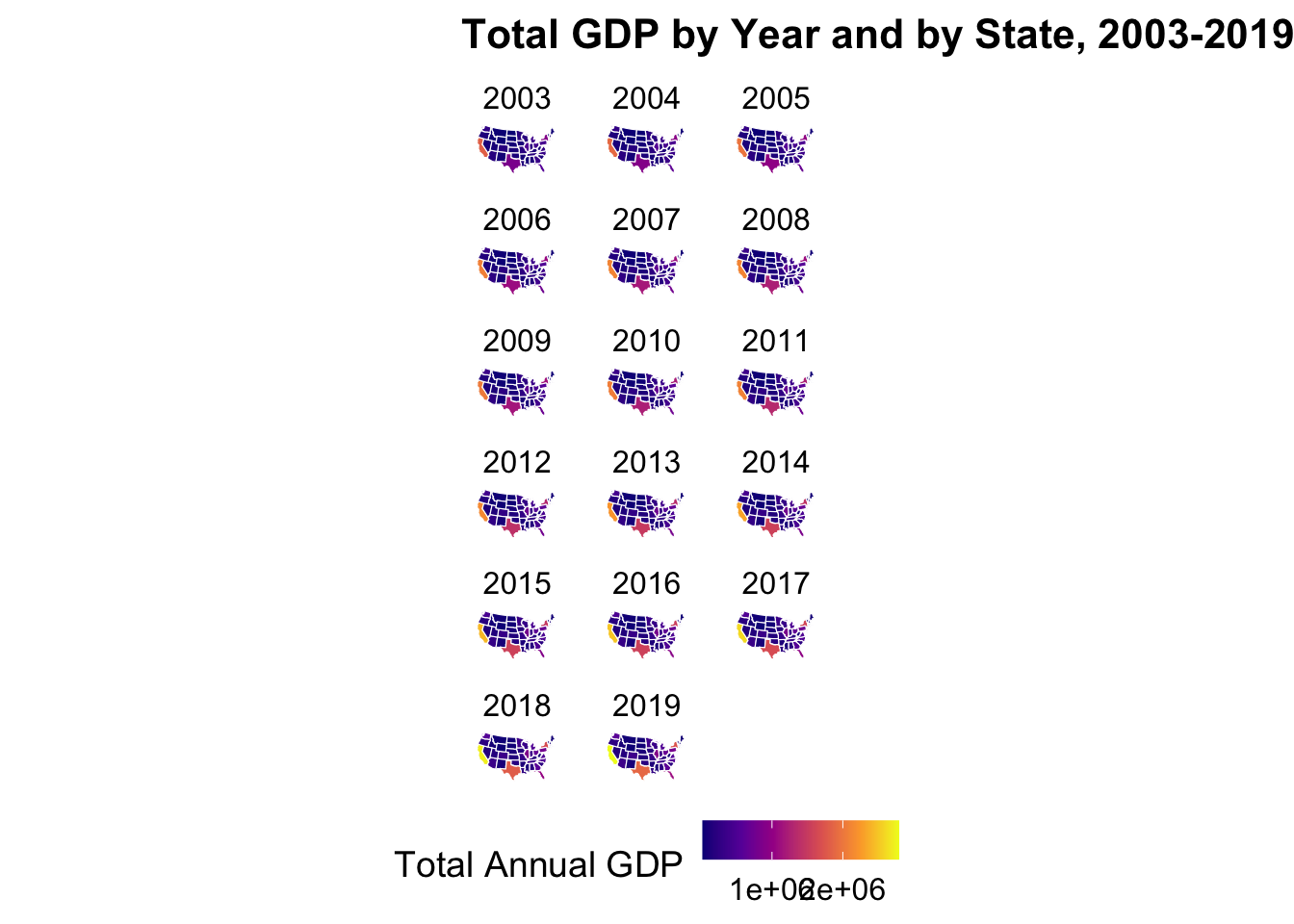
[This analysis was done to visualize Total GDP spread by state through years 2003 - 2019. Given the mass of data, the visualizations are a bit smaller than anticipated but general trends are: California has the highest total GDP of all states and this increases by the year as shown by the increased yellow tint, Texas appears to have the second highest total GDP in comparison with an increasing trend through the years.]
Total GDP by State by Year, A Heat Map
z = ztable(GDP_ALL)

makeHeatmap(z)
[This analysis is much easier to read than the map above. Using the heat map we can easily see that California has the highest GDP of all states for every year, followed by Texas and New York. The general trend is an increase in total GDP from 2003 to 2019.]