Stock Return and Risk Calculations
This post will center on simple stock portfolio risk and return analysis using R
Install all necessary packages.
#install.packages("tidyquant")
#install.packages("timetk")
#install.packages("plyr")
#install.packages("knitr")
#install.packages("dplyr")
#install.packages("quantmod")
#install.packages("BatchGetSymbols")
#install.packages("tsbox")
#install.packages("lubridate")

library("tidyquant")
library("timetk")
library("ggplot2")
library("plyr")
library("knitr")
library("dplyr")
library("quantmod")
library("BatchGetSymbols")
library("tsbox")
library("lubridate")
Downloading and Plotting Daily Return Data
#Data is downloaded using get_symbols function from quantmod
RSP <- getSymbols("RSP", src = "yahoo", from = '2003-04-30', to = "2020-07-07", auto.assign = FALSE)

RSP_Daily_Return <- dailyReturn(RSP)

#Daily Stock Prices are Plotted
RSP_Daily_Return %>%
  ggplot(aes(x = index(RSP_Daily_Return), y = daily.returns)) +
  geom_line(size=0.5, color="steel blue") +
  ggtitle("Guggenheim Invest S&P 500 Pure Value ETF since 2003") +
  scale_x_date(date_breaks = "years", date_labels = "%Y") +
  labs(x = "Date", y = "Adjusted Price")
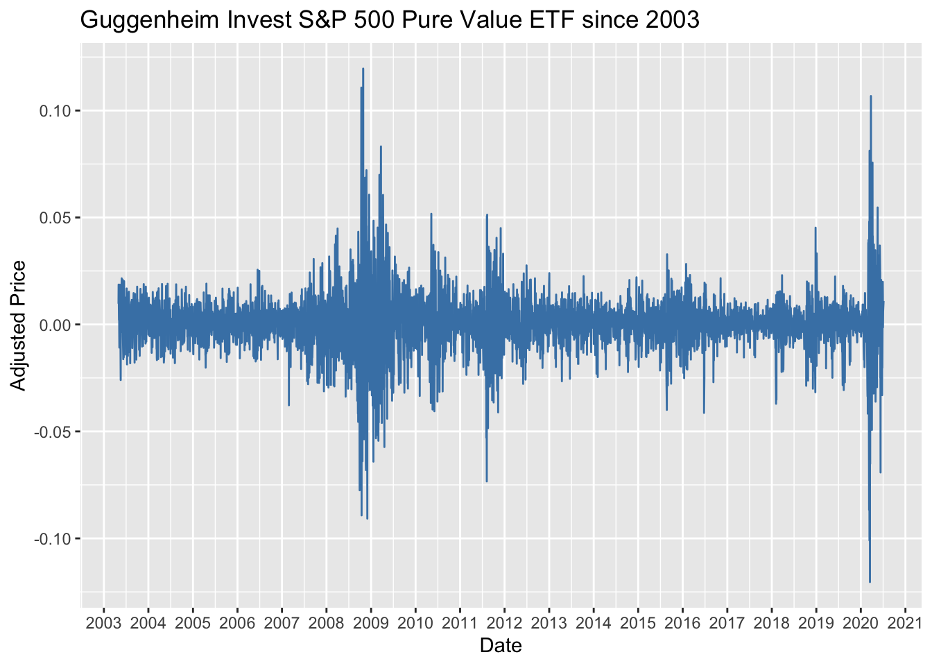
[ Graph of Daily Returns is difficult to interpret, but we see both extreme highs and lows during the 2008-2009 financial crisis as well as the highs and lows in 2020 during the COVID pandemic]
Viewing and Plotting Monthly Returns
#Share Price Data is already downloaded using the get_symbols function from quantmod.  Quantmod makes return calculations easy with monthlyReturn().
RSP_Monthly_Return <- monthlyReturn(RSP)

#Viewing data before analysis
head(RSP_Monthly_Return, n=10)
##            monthly.returns
## 2003-05-30     0.109405980
## 2003-06-30     0.008656778
## 2003-07-31     0.023535694
## 2003-08-29     0.043136238
## 2003-09-30    -0.019723212
## 2003-10-31     0.069236656
## 2003-11-28     0.021109961
## 2003-12-31     0.048780522
## 2004-01-30     0.023698842
## 2004-02-27     0.019039376
#Plotting Monthly Return Data.
RSP_Monthly_Return %>%
  ggplot(aes(x = index(RSP_Monthly_Return), y = monthly.returns)) +
  geom_line(size=0.5, color="orange") +
  ggtitle("Guggenheim Invest S&P 500 Pure Value ETF Daily Return since 2003") +
  labs(x = "Date", y = "Monthly Return")
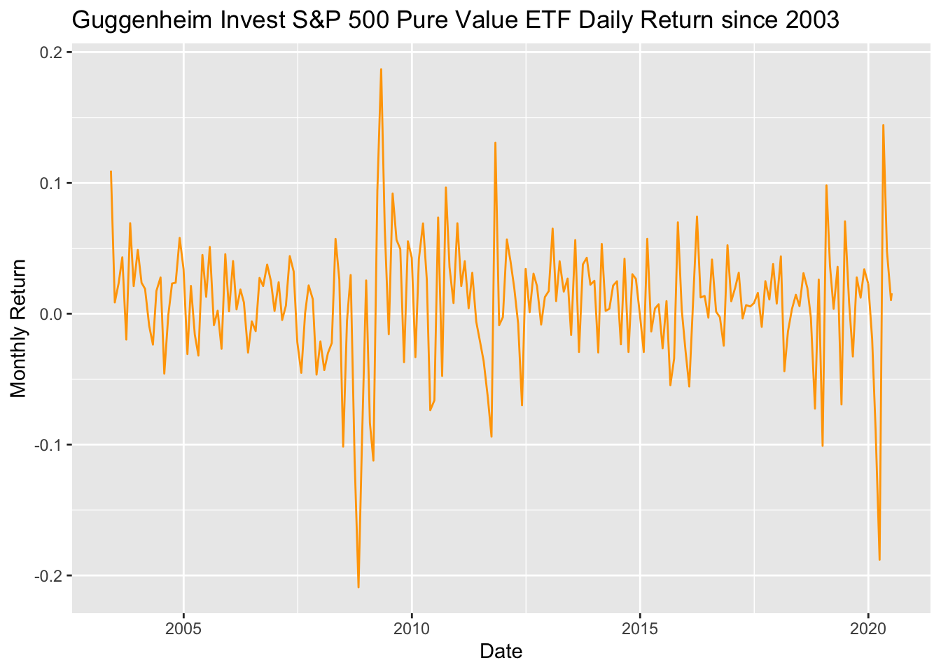
[The line graph for the monthly returns is easier to interpret than the daily return data. It appears monthly returns have been cyclical with extreme lows between the years 2008-2009 and the year 2020. Again these lows are due to both the 2008 financial crisis and the COVID pandemic respectively]
Calculating and Plotting Annual Returns
#Deriving Annula Returns. Using the yearlyReturn() function from quantmod
RSP_Yearly_Return <- yearlyReturn(RSP)

#Viewing the data
head(RSP_Yearly_Return)
##            yearly.returns
## 2003-12-31    0.341089069
## 2004-12-31    0.152897812
## 2005-12-30    0.062563958
## 2006-12-29    0.141204177
## 2007-12-31   -0.003379806
## 2008-12-31   -0.410767295
#Plotting Annual Returns with a Line Graph.
RSP_Yearly_Return %>%
  ggplot(aes(x = index(RSP_Yearly_Return), y = yearly.returns)) +
  geom_line(size=0.5, color="orange") +
  ggtitle("Guggenheim Invest S&P 500 Pure Value ETF Daily Return since 2003") +
  labs(x = "Date", y = "Annual Return")
#Plotting Annual Returns with Bar Graph
RSP_Yearly_Return %>%
  ggplot(aes(x = index(RSP_Yearly_Return), y = yearly.returns)) +
  geom_bar(stat="identity", color="orange") +  #stat=identity means bar represents value where as stat=bin would be equal to the number of cases which is not applicable in this case.
  ggtitle("Guggenheim Invest S&P 500 Pure Value ETF Daily Return since 2003") +
  labs(x = "Date", y = "Annual Return")
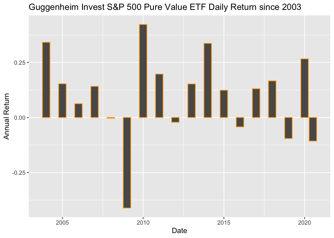
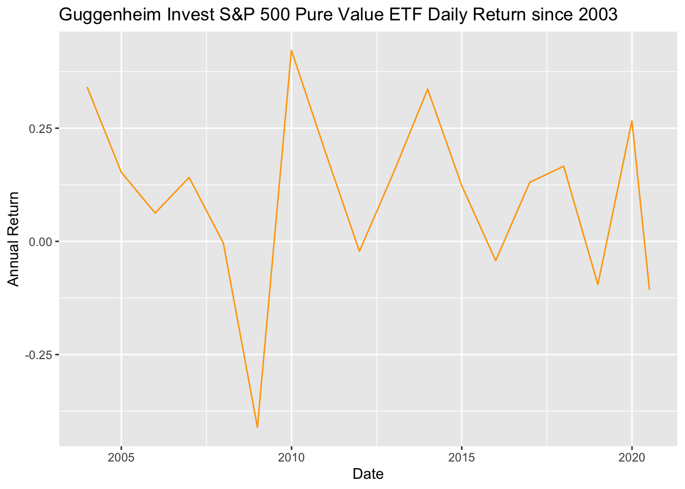
[Above are a line graph and a bar graph for RSP’s annual return data. The line graph appears to exhibit quite a bit of fluctuations with more extereme values during the financial crisis of 2008 and 2020 COVID crisis. For this type of analysis, the bar graph makes interpretation easier than the line graph. It is clear, both the magnitude as well as when such flucations in annual returns occurred]
Cumulative Daily Return for RSP
#Convert RSP_Daily_Return from an XTS or time series to a data frame so that we can mutate
RSP_Daily_Return <-  as.data.frame(RSP_Daily_Return)

#Converting the daily return variable into a numeric data type
daily.return <- as.numeric(RSP_Daily_Return$daily.returns)

#What if I wanted to know what the cumulative return for RSP was since 2003
RSP_Cumulative_Return <- as.data.frame(RSP_Daily_Return) %>%
            mutate(creturn = cumprod(1 + daily.returns)-1)  #(1 + r) * (1 + r)...

#Index functions converts the ref.date variable from an xts to a date variable.
RSP_Cumulative_Return$dates <- index(RSP_Daily_Return)

#1$ in 2003 would be around $4.7 today
RSP_Cumulative_Return %>%
  ggplot(aes(x = dates, y = creturn)) +
  geom_line(size=0.5, color="orange") +
  ggtitle("Guggenheim Invest S&P 500 Pure Value ETF Daily Return since 2003") +
  labs(x = "Date", y = "Cumulative Daily Return")
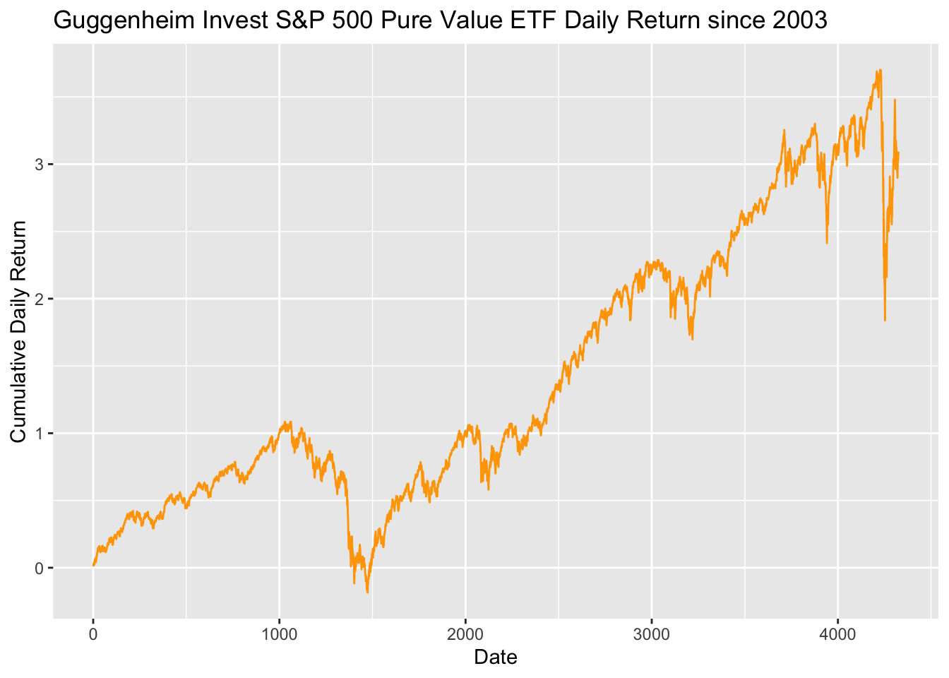
[$1 in 2003 would be around $3.5 today. ]
Downloading and Plotting Data for Multiple Stocks
#the ticker symbols for multiple stock are stored in the tickers variable
tickers <- c("RSP", "DIA", "AAPL", "DIS", "GOOG", "BAR", "UAL")

#Pricing and Return Data is downloaded through the BatchGetSymbols function.  Based on research I did online, this function appears to be the most efficient means of downloading stock data for muliple different stocks
multiple_stocks <- BatchGetSymbols(tickers,
                                   first.date = '2007-01-01',
                                   last.date = "2020-06-30",
                                   freq.data = "yearly", # calculates annual return data
                                   type.return = "arit",
                                   do.complete.data = FALSE,
                                   do.fill.missing.prices = TRUE,
                                   do.cache = TRUE,
                                   do.parallel = FALSE, be.quiet = FALSE)


#Its important to always look at your data before you analyze
head(multiple_stocks$df.tickers)
## # A tibble: 6 x 10
##   ticker ref.date    volume price.open price.high price.low price.close
##   <chr>  <date>       <dbl>      <dbl>      <dbl>     <dbl>       <dbl>
## 1 AAPL   2007-01-03 6.17e10       12.3       28.5      11.9        12.0
## 2 AAPL   2008-01-02 7.15e10       28.5       27.8      11.5        27.8
## 3 AAPL   2009-01-02 3.58e10       12.3       30.2      11.2        13.0
## 4 AAPL   2010-01-04 3.78e10       30.5       46.5      27.4        30.6
## 5 AAPL   2011-01-03 3.10e10       46.5       60.3      45.0        47.1
## 6 AAPL   2012-01-03 3.30e10       58.5      100.       58.7        58.7
## # … with 3 more variables: price.adjusted <dbl>, ret.adjusted.prices <dbl>,
## #   ret.closing.prices <dbl>
ggplot(multiple_stocks$df.tickers, aes(x = ref.date, y = price.adjusted, color = ticker)) +
  geom_line() +
  ggtitle("Price chart for multiple stocks")
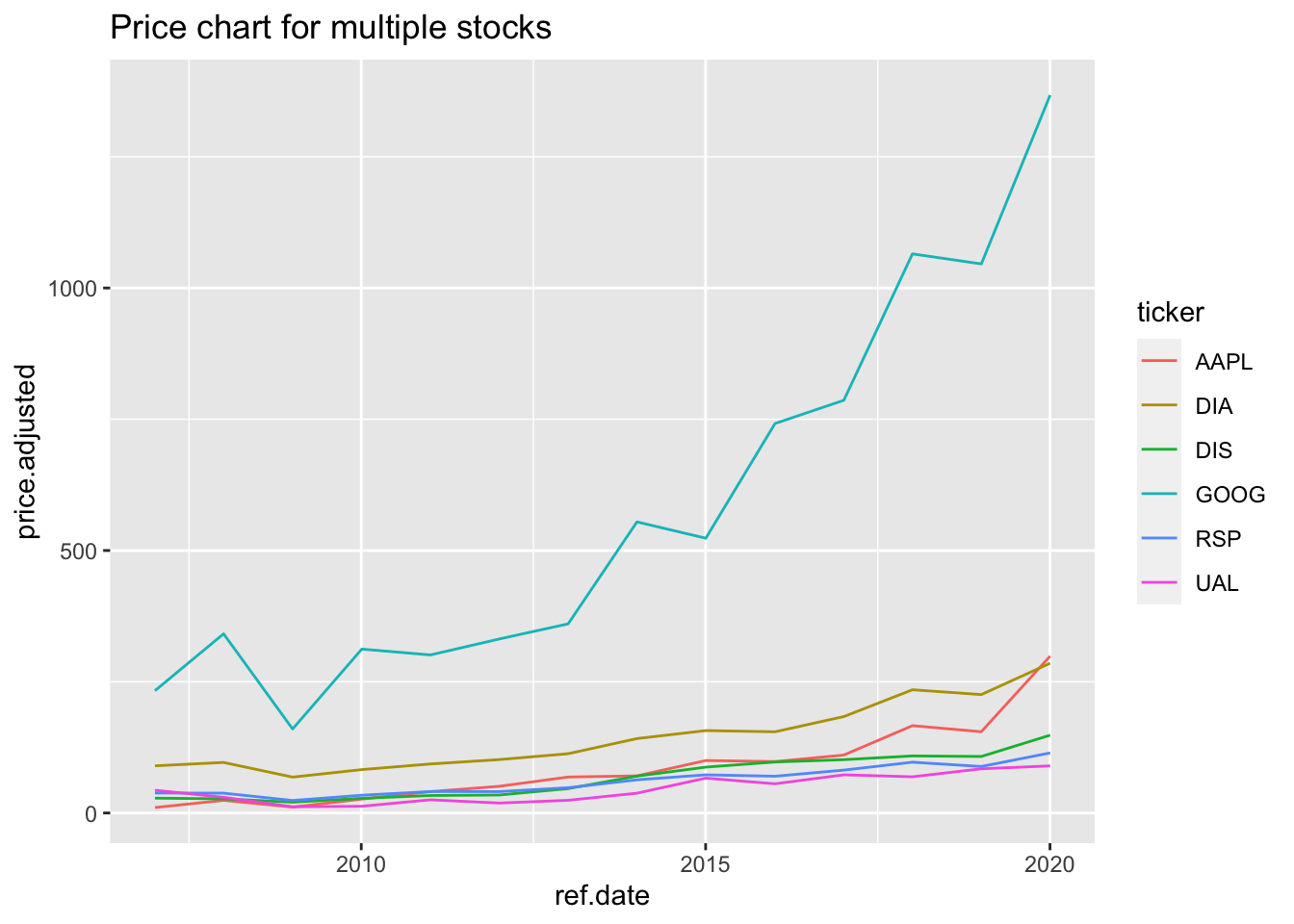
[This line graph is the pricing data for multiple stocks. Google has the highest stock price per share with around $1500 per share today. The next highest stock price today is Apple, with DIA, an Dow Jones ETF following.]
Plotting Daily Returns for Multiple Stocks
#Would like to investigate the cumulative return of several stocks simultaneosly
multiple_stocks_df <- data.frame(multiple_stocks$df.tickers)

head(multiple_stocks_df)
##   ticker   ref.date      volume price.open price.high price.low price.close
## 1   AAPL 2007-01-03 61748996400   12.32714   28.54714  11.89571    11.97143
## 2   AAPL 2008-01-02 71495301500   28.46714   27.84714  11.49857    27.83429
## 3   AAPL 2009-01-02 35813421700   12.26857   30.23428  11.17143    12.96429
## 4   AAPL 2010-01-04 37756231800   30.49000   46.49572  27.43571    30.57286
## 5   AAPL 2011-01-03 31014834900   46.52000   60.32000  45.04572    47.08143
## 6   AAPL 2012-01-03 32991051100   58.48571  100.30000  58.74714    58.74714
##   price.adjusted ret.adjusted.prices ret.closing.prices
## 1       10.36364                  NA                 NA
## 2       24.09607           1.3250593          1.3250596
## 3       11.22315          -0.5342334         -0.5342332
## 4       26.46683           1.3582365          1.3582369
## 5       40.75828           0.5399755          0.5399748
## 6       50.85724           0.2477768          0.2477774
#Looking at data before analysis
multiple_stocks_df %>%
  ggplot(aes(x = ref.date, y = ret.adjusted.prices)) +
  geom_line( aes(colour = ticker))  +
  ggtitle("Multiple Stocks Annual Arithmetic Return") +
  labs(x = "Date", y = "Annual Return")
## Warning: Removed 6 row(s) containing missing values (geom_path).
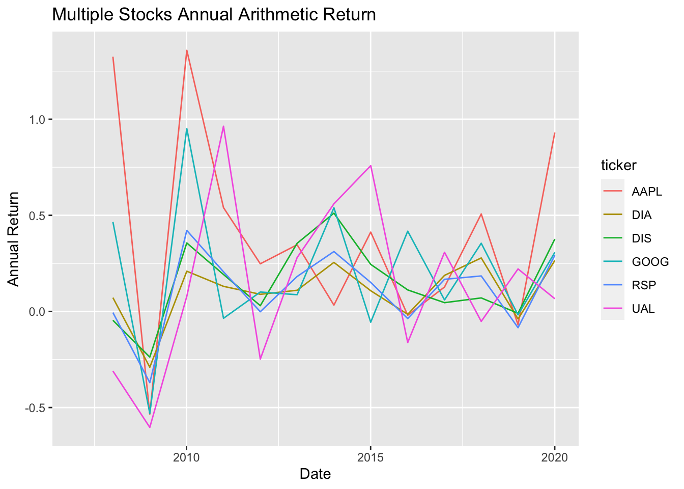 [Daily Return data is hard to interpret.]
Cumulative Daily Stock Return for Multiple Stocks
#Cumulative Stock Return for Multiple Stocks
multiple_stocks_daily <- BatchGetSymbols(tickers,
                                   first.date = '2007-01-01',
                                   last.date = "2020-06-30",
                                   freq.data = "daily",
                                   type.return = "arit")
##
## Running BatchGetSymbols for:
##    tickers =RSP, DIA, AAPL, DIS, GOOG, BAR, UAL
##    Downloading data for benchmark ticker
## ^GSPC | yahoo (1|1) | Found cache file
## RSP | yahoo (1|7) | Found cache file - Got 100% of valid prices | Feels good!
## DIA | yahoo (2|7) | Found cache file - Got 100% of valid prices | Looking good!
## AAPL | yahoo (3|7) | Found cache file - Got 100% of valid prices | Got it!
## DIS | yahoo (4|7) | Found cache file - Got 100% of valid prices | OK!
## GOOG | yahoo (5|7) | Found cache file - Got 100% of valid prices | Got it!
## BAR | yahoo (6|7) | Found cache file - Got 21% of valid prices | OUT: not enough data (thresh.bad.data = 75%)
## UAL | yahoo (7|7) | Found cache file - Got 100% of valid prices | Youre doing good!
#converting the df.tickers data package into a data frame
multiple_stocks_daily_ret_df <- data.frame(multiple_stocks_daily$df.tickers)

#Data that is missing or categorized as NA is replaced with a 0 to make analysis easier
multiple_stocks_daily_ret_df[is.na(multiple_stocks_daily_ret_df)] <- 0

#Need to check to see if NAs are replaced with 0s
head(multiple_stocks_daily_ret_df)
##   price.open price.high price.low price.close volume price.adjusted   ref.date
## 1      47.58      47.79     47.04       47.32 458900       38.05593 2007-01-03
## 2      47.27      47.48     47.04       47.39 323100       38.11223 2007-01-04
## 3      47.23      47.23     46.94       47.07 291500       37.85487 2007-01-05
## 4      47.01      47.23     46.89       47.17 279000       37.93529 2007-01-08
## 5      47.25      47.30     46.97       47.23 354500       37.98356 2007-01-09
## 6      47.10      47.42     46.97       47.37 249600       38.09615 2007-01-10
##   ticker ret.adjusted.prices ret.closing.prices
## 1    RSP         0.000000000        0.000000000
## 2    RSP         0.001479139        0.001479269
## 3    RSP        -0.006752453       -0.006752458
## 4    RSP         0.002124350        0.002124453
## 5    RSP         0.001272272        0.001272037
## 6    RSP         0.002964204        0.002964196
#Calculating the cumulative daily return using the cumprod function
cumulative_multiple_stocks_daily <- multiple_stocks_daily_ret_df %>%
            group_by(ticker) %>%
            mutate(creturn = cumprod(1 + ret.adjusted.prices)-1) #(1 + r) * (1 + r)...

#Looking at data before plotting.  Want to check to see if the cumulative product function worked correctly.
head(cumulative_multiple_stocks_daily)
## # A tibble: 6 x 11
## # Groups:   ticker [1]
##   price.open price.high price.low price.close volume price.adjusted ref.date
##        <dbl>      <dbl>     <dbl>       <dbl>  <dbl>          <dbl> <date>
## 1       47.6       47.8      47.0        47.3 458900           38.1 2007-01-03
## 2       47.3       47.5      47.0        47.4 323100           38.1 2007-01-04
## 3       47.2       47.2      46.9        47.1 291500           37.9 2007-01-05
## 4       47.0       47.2      46.9        47.2 279000           37.9 2007-01-08
## 5       47.2       47.3      47.0        47.2 354500           38.0 2007-01-09
## 6       47.1       47.4      47.0        47.4 249600           38.1 2007-01-10
## # … with 4 more variables: ticker <chr>, ret.adjusted.prices <dbl>,
## #   ret.closing.prices <dbl>, creturn <dbl>
#See Multiple Stock Cumulative Return
cumulative_multiple_stocks_daily %>%
  group_by(ticker) %>%  # Need to group multiple stocks
  ggplot(aes(x = ref.date, y = creturn, color = ticker)) +
  geom_line() +
  labs(x = "Date", y = "Cumulative Returns") +
  ggtitle("Cumulative returns for Multiple Stocks Since 2007") +
  scale_color_brewer(type = 'qual') +
  theme_dark()
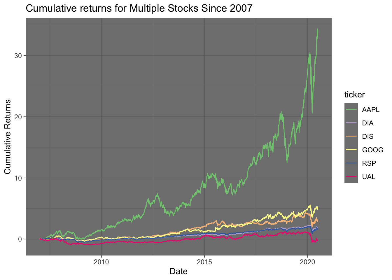
[Apple has the highest cumulative return compared to all the other stocks in the group. $1 of Apple at the beginning of 2007 is equal to $35 today]
Calculating the Standard Deviation for Multiple Stock
#Using the standard deviation function from R to find the SD of multiple stocks.  The SD is multiplied by the square root of 252 to annualized the data.  252 is the average number of trading days in a year.
Multiple_Stocks_SD_Table <-
cumulative_multiple_stocks_daily %>%
  group_by(ticker) %>%
  summarize(standard_deviation = round(StdDev(ret.adjusted.prices) * sqrt(252), digits=4) * 100)

#Looking at the data before plotting
head(Multiple_Stocks_SD_Table)
## # A tibble: 6 x 2
##   ticker standard_deviation[,1]
##   <chr>                   <dbl>
## 1 AAPL                     32.2
## 2 DIA                      20.2
## 3 DIS                      28.0
## 4 GOOG                     29.4
## 5 RSP                      22.7
## 6 UAL                      69.6
#Using Bar Graph to plot Mean Annual Return for Multiple Stock in Descending Order
ggplot(data = Multiple_Stocks_SD_Table, aes(x = reorder(ticker, -standard_deviation), y= standard_deviation)) +
geom_bar(stat="identity", fill= "blue", colour="orange") +
geom_text(aes(label = paste(standard_deviation, "%", sep = "")), nudge_y = 2) +
ggtitle("Multiple Stocks Mean Annual Arithmetic Returns Since 2007") +
labs(x = "Company", y = "Mean Annual Return")

[Stocks are arranged in order of descending riskiness. United Airlines has the highest level of risk with an SD of 69.6%, followed by Apple, Google, etc. Not suprising the RSP and DIA ETFs have the lowest risk out of this group of stocks given they represent the overall market]